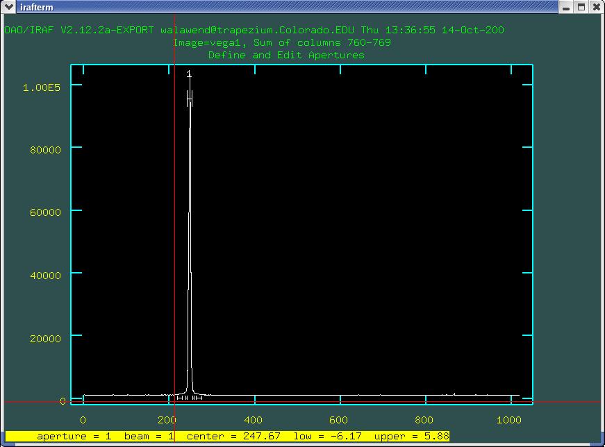
Fig. 1
NOTE: for a much more complete and detailed picture of spectral reductions, see the tutorial: A User's Guide to Reducing Slit Spectra with IRAF, by Phil Massey, Frank Valdes, and Jeannette Barnes at NOAO.
The first steps in reducing spectra are identical to reducing images: perform dark and flat field correction as described in section V. A. - F. We then need to combine our spectra, however we cannot use the same alignment procedure as with images in section V. G.
NOTE: When flat fielding, if the spectral flat is not high signal to noise, then don't use it. Often the small systematics in CCDs are not worth adding extra noise from the flat field.
After generating a final combined spectrum, we will then generate a wavelength solution, which means that we will determine the mapping between pixel number along the spectrum and wavelength.
It may be necessary to define the dispersion axis. This is
controlled by the DISPAXIS keyword in the header. Check the header by
using the imhead task with the long keyword set:
cl> imhead science_exposure_filename long+
Look for the DISPAXIS keyword in the output. Additionally one
could also use the UNIX grep command to pick out the
DISPAXIS keyword:
cl> imhead science_exposure_filename long+ | grep DISPAXIS
grep is case sensitive so be sure to capitalize
accordingly (or use the -i option with grep).
For a spectra with the dispersion axis horizontal, DISPAXIS should be 1, for vertical spectra, DISPAXIS should be 2.
If the DISPAXIS header keyword needs to be altered or added, use
the hedit task:
cl> hedit science_exposure_filename DISPAXIS 1 add+
If your spectra is vertical, use 2 as the value for DISPAXIS in
hedit.
Note: I've put the add keyword in explicitly, it is only necessary if the DISPAXIS header keyword doesn't exist in the image.
NOTE: The apall procedure for extracting the trace of the spectrum is primarily designed for continuum spectroscopy. It may be possible to use it with nebular spectroscopy, but I won't go into that here. In this tutorial, it is assumed that we are working with a continuum spectrum. If you are working with a nebular spectrum, then parts C-G should be replaced by another method (e.g. see the IRAF tutorial linked at the top of this page). One simple method is described here.
apall is a multi-step task which defines and extracts
the data from your 2D CCD image. To access apall, load
the noao, onedspec, twodspec,
and apextract packages:
cl> noao

cl> onedspec

cl> twodspec

cl> apextract
Now we must edit the apall parameters:
cl> epar apall


PACKAGE = apextract

   TASK = apall


input   =                      List of input images

(output =                    ) List of output spectra

(apertur=                    ) Apertures

(format =           multispec) Extracted spectra format

(referen=                    ) List of aperture reference images

(profile=                    ) List of aperture profile images


(interac=                 yes) Run task interactively?

(find   =                  no) Find apertures?

(recente=                  no) Recenter apertures?

(resize =                  no) Resize apertures?

(edit   =                 yes) Edit apertures?

(trace  =                 yes) Trace apertures?

(fittrac=                 yes) Fit the traced points interactively?

(extract=                 yes) Extract spectra?

(extras =                 yes) Extract sky, sigma, etc.?

(review =                 yes) Review extractions?


(line   =               INDEF) Dispersion line

(nsum   =                  10) Number of dispersion lines to sum or median
change find to no, recenter to no, and resize to no (as I have them above).
NOTE: apall has many parameters, I've only shown the
first page of them here.
Also we need to edit the apextract parameters:
cl> epar apextract

PACKAGE = twodspec

   TASK = apextract


(dispaxi=                   1) Dispersion axis (1=along lines, 2=along columns)

(databas=            database) Database

(verbose=                  no) Verbose output?

(logfile=                    ) Text log file

(plotfil=                    ) Plot file

(version= APEXTRACT V3.0: August1990)

(mode   =                  ql)

($nargs =                   0)
change dispaxis to 1 (along lines).
To run apall and extract a spectrum:
cl> apall science_exposure_filename
this will bring up an interactive window where one can define the various apertures:

this is a plot of pixel values as a function of y, a stellar
spectrum is represented by the peak (in this case around line 250 or
so). We want to set an aperture which gathers all of the light in
that peak. First we need to zoom in on that spectrum. To do this we
use the w and e commands. Type
w to zoom, then use e to define the lower
left and the upper right of the region we want to zoom in on. For
example, if I typed w then e at the location
of the cursor showing in Fig. 1, and then typed e again
after pointing to the upper right of the peak, I would get what is
shown in Fig. 2. You can use the key combination w a to
reset the zoom to default.
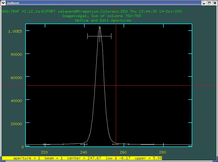
now we can see in more detail. The region outlined by the bar with
the numeral 1 above it is a automatically defined aperture which has
been selected by IRAF. In this case it looks reasonable, but let's go
though the exercise of redefining it. We can define the center of the
aperture either using the cursor (point to the center and type
n) or by using the cursor as a starting point and having
IRAF centroid the profile (point near the center and type
m). You can use the d key to delete
previously defined apertures (each aperture will be numbered 1, 2, 3,
etc.). The width of the aperture can be defined using the
y key, which sets the width to whatever the width is at
the y position that the cursor is pointed at (experiment with this to
get a feeling for how it works). Conversely you can set the upper and
lower boundaries to the width of the aperture using the u
and l keys (for upper and lower boundaries
respectively).
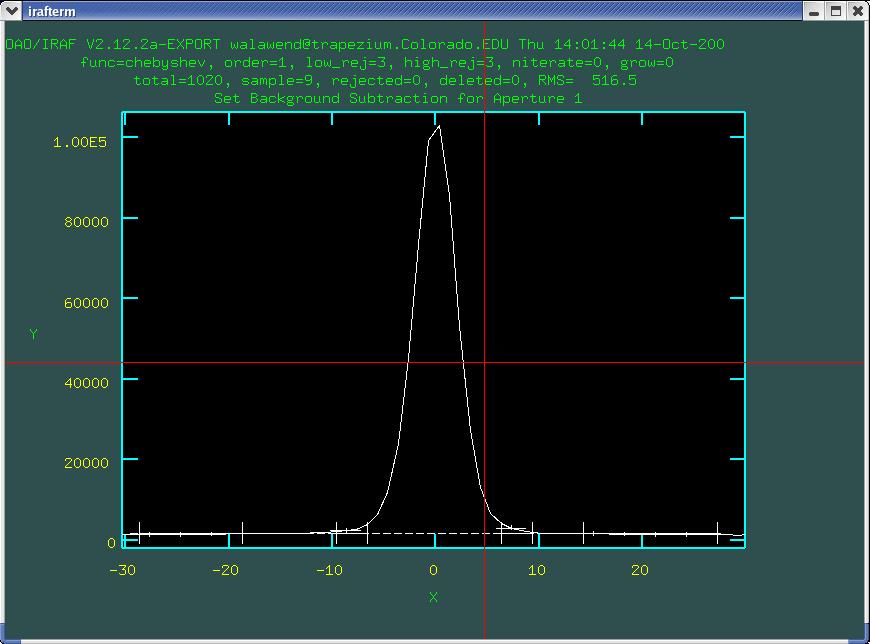
Once you have set the aperture, hit b to move on to
setting the background apertures. Again there will be a preselected
fit by IRAF there for you as in Fig. 3.
I would recommend setting a wider view which emphasizes the
background using the w e e and w a commands
as shown in Fig. 4.
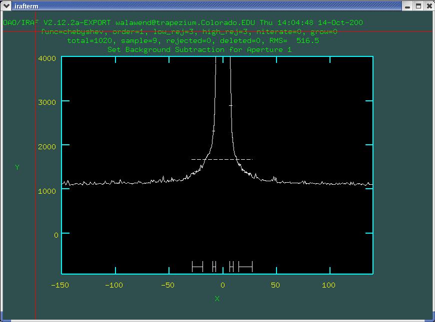
Now we can see the background. Those four horizonatal lines at the
bottom define the region where the background is being sampled. The
horizontal dashed line is the fit which is obviously incorrect, so
we'll need to redefine the background sections. We can use the
s key to set new regions to be used in the background
fit. press the s key at either end of the region you
want to use for the background fit then hit the f key to
perform the fit and the dashed line should move (you can delete
previously defined fitting regions with the z key). I
would recommend using a large swath of background on either side of
the aperture as seen in Fig. 5.
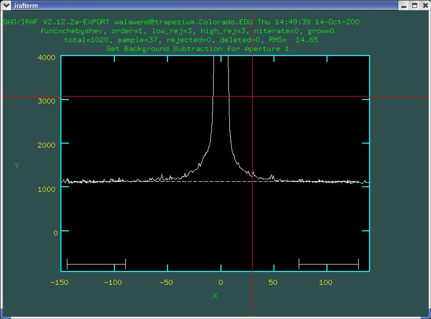
Now you can see that the background fit (dashed line) accurately
represents the background. Once you are satisfied with the background
fit, type q to return to the aperture edit mode.
The trace is what determines the shape of the aperture as you move along the dispersion axis. For example if your stellar spectrum is not horizontal or if it is curved, IRAF needs to determine its shape to accurately extract the spectrum.
Hitting q in the aperture edit mode will take you to
the trace fit as seen in Fig. 6:
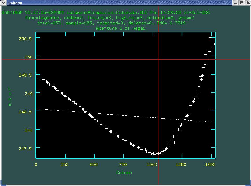
Here the data points (plus signs) represent the trace of the
spectrum and the dashed line indicates the fit. The difference looks
dramatic until you realize that the y-axis of this plot is just 3
pixels high, so the deviation from the straight line fit is just a few
pixels. To increase the order of the fitted polynomial, use the
:or command (don't forget the colon). After typing
:or enter the order of the polynomial you want to fit.
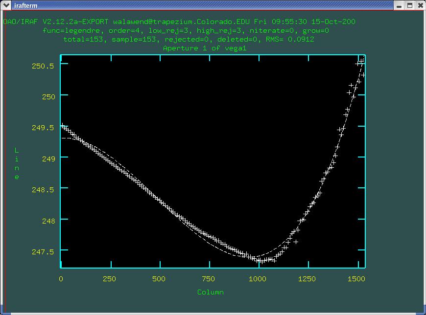
In this case I'll use 4th order and then hit f to perform
the fit, and you can see that the fit tightens up nicely (Fig. 7).
The fit still isn't prefect, but we are within about 0.1 pixels
everywhere along the trace.
All of the apertures we've just defined are stored in a file called
database/apscience_exposure_filename in the
current directory. This way you can come back to this image later and
still retain the aperture definitions. To work on another exposure
but using the same apertures you can use apall as
cl> apall science_exposure_filename2 ref=science_exposure_filename
To extract spectra from your data, hit q to quit the
trace fitting routine and answer the questions asked by apall.
There are two options for extracting the spectrum. First, one can
simply add up all of the counts in the aperture and subtract off the
background. This however, has a couple of potential problems. One is
that small numbers of photons in the wings increase the noise.
Another is that cosmic ray hits can throw off the sum. The second
option is a variance weighting in which the sum is weighted by the
signal to noise in that pixel. This method is more resistant to a few
noisy pixels and does a pretty good job rejecting cosmic rays. The
disadvantage is that the method assumes only read noise (no dark
current noise) and you have to explicitly enter the gain and read
noise in epar apall.
Your extracted spectrum will be written as a one dimensional
spectrum in the file
science_exposure_filename.ms.fits.
IRAF has a routine for generating a wavelength calibration solution
using a list of line wavelengths in your calibration lamp exposure. I
have taken the SBO calibration lamps and generated this list
(sbo_HeAr.dat). Use the identify task to associate these
lines with features in your calibration lamp exposure.
cl> identify cal_lamp_exposure_filename section='line l1 l2' coordlist='path/sbo_HeAr.dat'
The l1 and l2 parameters are the lines
which will be averaged to generate the spectrum (since this is a
wavelength calibration we will not worry about extracting a detailed
aperture and just use the lines).
It has come to my attention that the section='line l1
l2' may not work properly. If it appears that the lines are
not being averaged properly, you can use the method for adding lines
described in the alternative to
apall page to average the lines in the calibration
exposure.
Use the calibration lamp plots from the SBO manual
to identify two or three lines, point the cursor at the centers of
these lines and hit m (for mark) and enter the
wavelengths as requested. Hit f to fit a rough
wavelength solution. Hit q to return to the display of
the spectrum. Now that IRAF has a rough idea of what the solution is,
it can look at the line list and identify additional lines in your
spectrum and determine their wavelengths from the sbo_HeAr.dat
database. This will give several more point in the fit to the
function relating wavelength to pixel number. To have IRAF
automatically identify additional lines, hit l.
Now we have to check whether IRAF's automatic identification worked
properly. Use the z,d,+,p keys to eliminate any false markings (see
the identify help page for more info). Hit f again to
fit the wavelength solution with the new markings. Use d to delete
any outlier points in the fit. When you are satisfied with the fit,
hit f, and then quit the IDENTIFY program (hit q twice).
You have now generated a wavelength solution which is probably stored
in a subdirectory called database.
Now we need to associate that wavelength solution with the science
exposures to which it applies. To do this we add a keyword to the
science exposure header. To modify a header use the
hedit task (be sure to apply it to the file that was
output from apall):
cl> hedit science_exposure_filename.ms REFSPEC1 "cal_lamp_exposure_filename" add+
If the header field REFSPEC1 already exists in the header, use add-
Now to apply the wavelength solution to the image using the dispcor task:
cl> dispcor science-exposure-filename calibrated-science-exposure-filename
Now you can use splot to inspect and analyze your data
with a dispersion axis in units of angstroms rather than pixels.
We will use splot to view the calibrated spectrum. If
you have properly used identify and dispcor
then the horizontal axis of the splot window should be in wavelength
units (angstroms). If you move the curson over a point on the
spectrum and hits space, then splot will print out the coordinates of
the cursor at the bottom of the screen
The splot task has a number of interactive tools for
analyzing your spectrum. As with most interactive IRAF tasks hitting
the ? key brings up a short help page on the interactive
commands. We'll go through a few of the most useful commands one at a
time.
You can rescale the axis and "zoom in" on a particular section of
spectrum by using the a key to deliniate the corners of a
box you would like to zoom in to. Point the cursor at the part of the
spectrum that you would like to be in the lower left corner of the new
view and hit a. Then point at the upper right corner and
hit a. The view will zoom to a box defined by the points
you specified.
To redraw the screen and zoom out to the full view, simply press
c.
One other command which can be useful is the :hist
command. This simply toggles between two different line types for the
plot. Turning it on goes to a historgram style line plot, otherwise
each point in the spectrm is simply connected by a straight line in
the plot. Test out both to see which you prefer (Fig. 11 below is in
the default style, not histogram style).
In many cases you will want to determine the exact wavelength of
line center and the integrated flux in a line. To do this we must fit
a line profile to the data, sometimes several line profiles. The
deblend command in splot is a quick and easy way to do
this. Deblending is a multi-step process, so we'll go through it one
step at a time.
First, use the a key to zoom in on the line(s) you
wish to study.
Second, point the curson at a point in the continuum well to the
left of the lines and hit d, then point at a point in the
continuum well to the right and hit d again. This
defines the continuum level. Choosing how far away from the lines to
select can be tricky. You want to grab a large enough segment of
continuum, so that its level can be fit accurately, however the fit is
simply a lines with some slope, so if your continuum is non-linear,
you'll need to select a smaller segment which is approximately
linear. At the end of the fitting process we'll see a graphical
representation of the background fit, so you can check that the fit is
reasonable then.
Third, now we need to select which features in the spectrum to
fit. You'll notice that at the bottom of the splot
window, you get a menu saying something like:
Lines ('f'ile, 'g'aussian, 'l'orentzian, 'v'oigt, 't'ype, 'q'uit:
What you need to do is point the cursor at a line (you only need to
line up horizontally with the line, where you point vertically does
not matter) and hit a key indicating which type of line fit you'd like
to do. Let's do the simple example of fitting a gaussian, so we'll
point at a line at hit g. Do this for all lines in the
deblending segment that you defined with the d key even
if you are not interested in the properties of those lines. If you do
not fit a line, then those values will be assumed to be part of the
background and may throw off the background fit. Each time you
indicate a line to fit with, for example, the g key, it
will be marked with a short vertical line. Once you have marked all
the lines you want to fit, hit q to quit and move on to
the next deblending step. Once you do that, you will see a question
at the bottom of the splot screen:
Fit positions (fixed, single, all, quit)
IRAF is asking whether you want the centers (positions) of the
lines to be a variable in the fit. Unless you have some reason not to
do this, hit a, to indicate that you want all of the line
positions to be variables in the fit.
Now you will be confronted with a new question:
Fit Gaussian widths (fixed, single, all, quit)
Now it is asking whether the widths of the lines should be a
variable in the fit. Note, this question may vary depending on which
type of profile you used to mark the lines. For most purposed,
hitting a to indicate that all lines should have their
widths fit is a good choice.
Again you will be confronted with a new question:
Fit background (no, yes, quit)
IRAF is asking whether it should fir the background (or continuum)
flux. In most cases, you want to hit y for yes, fit the
background.
Now IRAF will dislay the results of the fit as shown in Fig. 11. First check to see that the fit is reasonable. The green dashed line shows the fit of the background level. You want this to be a good measurement of the average, in Fig. 11 this looks reasonable since the green line goes through the noise at a reasonable level. The red dashed lines show the line profiles that have been fitted. Do they roughly match the lines in the spectrum?
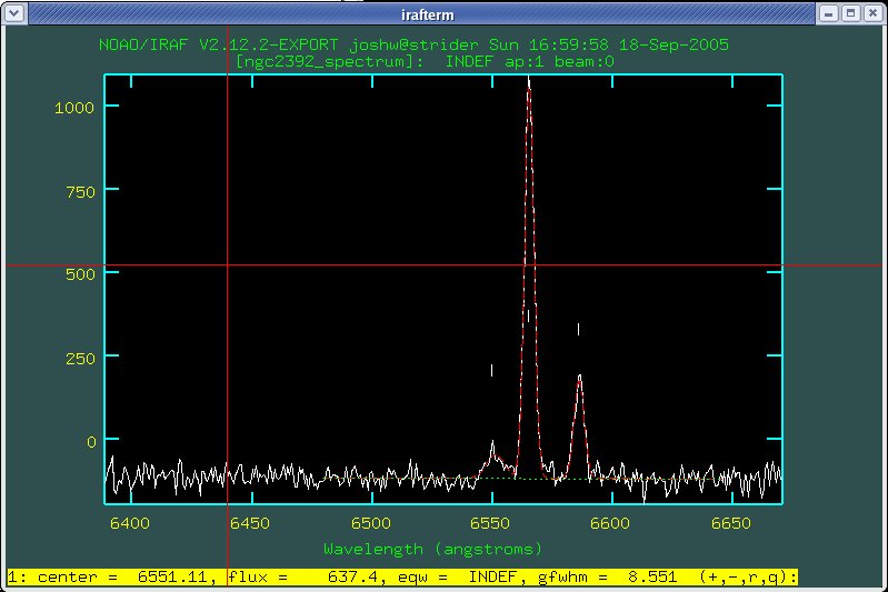
The line of text at the bottom of the splot window
gives you information about the fitted lines numbered 1 though n from
left to right. In Fig. 11 we see that the low, noisy, broad line on
the left is centered at 6551.11 angstroms, has a flux of 637.4 (this
is a measurement of the area under the line, so the units are
counts*angstroms), the equivalent width is undefined (INDEF) because
this is an emission line, not an absorption line, and the Gaussian
FWHM is 8.55 angstroms. To see the same information about the other
two lines you can use the + and - keys to
cycle through lines 1, 2, and 3. Pressing the r key
prints out the RMS noise of the background for comparison to the flux
in the lines.
Pressing q will quit these results. You may be asked
several of the previous questions again to see if you want to try the
fit with different parameters. To exit deblending, hit q
for each of these questions. When you have exited deblending you will
see a Deblending done message at the bottom of the screen
and you are back in regular splot, hitting q
again will exist splot completely.